Evaluation of Recent Statistical Methods for Detecting Differential Methylation Using BS-seq Data

Chenggong Han ^{1, †}, Hancong Tang ^{1, †}, Shuyuan Lou ^{1, †}, Yuan Gao ^{1, †}, Min Ho Cho ², Shili Lin ^{1, 2, *}

1. Interdisciplinary Ph.D. Program in Biostatistics, The Ohio State University, 1958 Neil Avenue Columbus, OH 43210-1247, USA
2. Department of Statistics, The Ohio State University, 1958 Neil Avenue Columbus, OH 43210-1247, USA

† These authors contributed equally to this work.

*   Correspondence: Shili Lin

Received: May 23, 2018 | Accepted: September 12, 2018 | Published: October 15, 2018

OBM Genetics 2018, Volume 2, Issue 4 doi:10.21926/obm.genet.1804041

Academic Editors: Stéphane Viville and Marcel Mannens

Special Issue: Epigenetic Mechanisms in Health and Disease

Recommended citation: Han C, Tang H, Lou S, Gao Y, Cho MH, Lin S. Evaluation of Recent Statistical Methods for Detecting Differential Methylation Using BS-seq Data . OBM Genetics 2018;2(4):041; doi:10.21926/obm.genet.1804041.

© 2018 by the authors. This is an open access article distributed under the conditions of the Creative Commons by Attribution License, which permits unrestricted use, distribution, and reproduction in any medium or format, provided the original work is correctly cited.

1. Introduction

DNA methylation plays a critical role in controlling gene expression and is also related to many aspects of cell processes, such as embryonic development, genomic imprinting, X-chromosomal inactivation, and preservation of chromosome stability [1]. While DNA methylation is vital for normal cell development, aberrant DNA methylation may also occur [2]. Such aberrant events, especially those that occur in the promoter region, may cause unexpected gene silencing, which is believed to be related to cancer [3]. It has been shown that methylation levels of neighboring CpG (or CG) sites may be spatially correlated [4], and it is further recognized that some particular genes in cancer cells have a higher probability of being hypermethylated, while there are others that tend to be hypomethylated [5]. As such, through studying DNA differential methylation, we can better understand how variation in DNA methylation is related to diseases such as various types of cancer.

In recent years, the role of DNA methylation in biological processes has been studied in greater extend. Evidence has suggested that DNA methylation may impact the global structure of the genome in the nucleus instead of directly affecting gene expression [6,7], providing a new perspective. Researchers have also shown that DNA methylation may be associated with gene activation, splicing [8], nucleosome positioning, and cellular plasticity [9]. The role of DNA methylation in biological and molecular processes remains a highly pursued research topic and is far from being fully understood.

A number of molecular methods for measuring genome-wide DNA methylation have been developed and can be divided into two main categories: microarrays and sequencing. Such methods may be further classified by the different molecular techniques that they use, including methylation-specific enzyme digestion (ED), affinity enrichment (AE), chemical treatment with bisulfite (BS), or a combination of these [10]. In particular, BS was a major breakthrough in measuring DNA methylation, which uses sodium bisulfite to convert unmethylated cytosine to uracil while leaving the methylated ones unchanged [11]. Coupling BS with microarray or sequencing enables genome-wide profiling of DNA methylation.

Different approaches have advantages and disadvantages in terms of coverage and cost. Methods based on whole genome sequencing have the highest coverage but are costly. Specifically, whole-genome bisulfite sequencing (WGBS) is the current gold standard, but is very expensive as BS conversion and sequencing are performed on the entire genome. On the other hand, reduced representation bisulfite sequencing (RRBS) considers only a subset of the CG sites in the genome, therefore, it is more economical, although still costly. However, its coverage is greatly reduced compared to WGBS, although still much greater coverage than its microarray counterpart. Together, WGBS and RRBS are referred to as BS-seq, and they constitute the state-of-the-art BS-based sequencing platforms. In addition, single molecule real-time BS (SMRT-BS) is an alternative that also has the multiplex feature for studies analyzing long read sequences [12].

Due to their cost, sample sizes from BS-seq experiments are typically very small (e.g. three cases versus three control samples), necessitating the use of analytical methods that are different from those for epigenome-wide association studies (EWAS), which primarily make use of microarray data. Despite the cost, BS-seq methods have gained a great deal of attention and interest in recent years, and they are the methods of choice when whole-genome profiling of DNA methylation is necessary. Therefore, statistical methods specifically designed for analyzing BS-seq data are indispensable.

In response to this need, a number of statistical methods have been developed in recent years specifically for analyzing BS-seq data, with the goal of identifying differentially methylated loci or differentially methylated cytosines (DMCs) and differentially methylated regions (DMRs). Such methods include BiSeq [13], DSS [14], MethylSig [15], RADMeth [16], BSmooth [17], BCurve [18], and others as described in a number of recent review papers [10,19,20,21,22,23], which will be discussed further in Section 5.

In this paper we focus on evaluating four methods (BiSeq, DSS, MethylSig, and RADMeth) to compare and contrast their performance on both DMC and DMR detection. The commonality of these methods is that they all rely on the use of both binomial and beta distributions for describing the observed data: the use of the binomial distribution is natural as the methylated reads among all reads at a CG site follow such a distribution, whereas the beta distribution is used to capture between-sample variability of the methylation levels within a group. This latter feature sets them apart from traditional statistical methods such as the Fisher exact test, which cannot naturally account for between-sample variability, although they can be more efficient for data without biological replications or with little variability. On the other hand, although these four methods share the commonality of accounting for variability between biological replicates, each method is unique in parameter estimation, data fusion (among neighboring CG sites), and covariate incorporation. These methods will be loosely referred to as “beta-binomial” based hereafter.

The reason that these four methods are chosen in this paper is that they are all “beta-binomial” based in the sense described in the previous paragraph. Such a type of approach appears to be the method of choice in many current studies, yet, their appropriateness and relative performance are still not fully understood. Although several recent review papers all described (at least some of) these methods [10,19,20,21,22,23], they mainly focused on features of the methods; any comparisons are largely descriptive rather than actual performance comparisons via simulation studies or real data analysis, with one exception. The exception is a very recent paper [21] that did compare among several methods, including the four that are the focus of the current paper. However, the simulation model, which used the negative-binomial distribution to generate the coverage and then used the binomial distribution for the methylated reads given the coverage may be too simplistic, leading to no appreciable benefits for beta-binomial based methods compared to the simple Fisher’s exact test or logistic regression analysis. Comparisons between some of these four methods have also been carried out elsewhere [16,20,22], though it is difficult to aggregate results of such evaluations since different comparisons were based on different sets of methods and simulation models with varying evaluation criteria. Most detrimentally, the said evaluations largely used data simulated from models that were the same as the analysis models for new methods being proposed; thus, the results may be biased toward the proposed new methods in the papers. To avoid such a pitfall, in this study we provided an objective evaluation of the four methods based on simulated and real data from both the WGBS and RRBS platforms. In particular, to be as unbiased as possible, our simulations take into account characteristics of real data, various levels of between-sample variation, and they do not use the specific models proposed in any of these four methods.

2. Materials and Methods

In the following, we describe each of the methods that will be compared in this paper, noting their common as well as unique features, including distribution, filtering, testing, covariate handling, “smoothing”, and “window-based” characterization. Although many of the features are self-explanatory and will be described in each individual method, a couple of the features deserve explanation here. In particular, by “smoothing”, we refer to whether information from nearby CpG sites is borrowed to improve the accuracy of data or parameter estimates. On the other hand, although all methods have some features that may be described as “window-based”, they differ in the details on how windows are defined and how information within a window is utilized. These features will be described in each of the methods where appropriate, with easy-to-read summaries provided in Supplementary Table S1.

2.1. BiSeq

BiSeq is an approach that enables detection of DMCs and DMRs through a two-stage procedure [13]. To execute this procedure, CpG clusters are obtained first: the algorithm scans the genome to divide it into regions such that within each region the neighboring CpG sites are less than 100 base pairs (bp) apart; a region is retained as a CpG cluster if it contains at least 20 CpG sites. Secondly, analyses are performed using methylation data within each CpG cluster via a smoothing function on the means of the binomial distributions through kernel smoothing.. For a given CpG site in a CpG cluster, the corresponding weighted local likelihood for its methylation level is maximized. The resulting methylation level, which is between 0 and 1, is taken as the methylation level at that position. This method then assumes that the smoothed methylation level follows a beta distribution and fits a beta regression with the group (disease or control) and other predictors (covariates) as explanatory variables.

A Wald test is conducted to test the group effect at each CG site. Based on the p-values from the Wald tests for all the sites within a CpG cluster, a two-stage procedure is conducted to ascertain whether the CpG cluster is a DMR (first stage) and if necessary, to find the DMCs within the cluster afterwards (second stage). Thus, one may view BiSeq as a window-based approach. Specifically, the first stage aims to detect “non-null” clusters by controlling the cluster-wise false discovery rate (FDR); the weighted Benjamini–Hochberg procedure at level q [24] is applied to the site-wise p-values to evaluate whether a cluster-wise FDR is below the set threshold q. During the second stage, a procedure is applied to control location-wise FDR at level q*. For each CpG site in “non-null” clusters (i.e. CpG clusters that pass the FDR threshold q in stage 1), its p-value is estimated, conditional on the fact that it belongs to a non-null cluster. The sites that are below the site-wise FDR threshold q* are then declared as DMCs. Adjacent DMCs with the same directionality (all hypomethylated or hypermethylated) are then linked to obtain DMRs.

2.2. DSS

A lognormal-beta-binomial empirical Bayes model is proposed in DSS [14]. First, the methylation reads of a sample at each site are assumed to follow a binomial distribution. To capture the biological variation among replicates, the mean methylated proportions across the samples at each CpG site are assumed to follow a beta distribution. The dispersion parameter of this beta distribution captures the variation of methylation proportions across samples (i.e, biological variation) relative to the group mean. In the DSS package, the dispersion parameters of the two conditions may be assumed to be the same or different. Although this beta-binomial model does not account for any other covariates, a more recent update called DSS-general does take covariates into consideration through regression modeling [25].

An empirical Bayes approach is taken, and in particular, a log-normal prior is assumed for the between-sample dispersion parameter. This log-normal prior selection does not appear to lead to sensitivity based on the simulation study using other prior distributions [14]. To completely specify the prior, the following empirical procedure is used to find the mean and variance of the log-normal distribution. First, the method of moments (MOM) is used to estimate the dispersion parameter at each CG site assuming the beta-binomial distribution for the observed methylation data. Then, the mean and variance of the logarithms of the MOMs across all CG sites are computed and used as the mean and variance of the log-normal prior. This may be considered as a window-based procedure for specifying the priors where the “window” is the entire genome. The conditional posterior distribution of the dispersion parameter at each site (given the mean estimate) is then maximized, leading to an empirical Bayesian estimator that takes the dispersions of other sites throughout the genome into consideration. This “shrunken” method gives a stable estimation of the variance.

A Wald test is then performed to find DMCs. For technical reasons, DSS filters out a locus when the coverage in all replicates in one condition is zero. To find DMRs after the identification of DMCs, DSS sets the following criteria: a DMR needs to exceed a minimum length (default is 50 base pairs in the package), the number of CG sites should be greater than a user-specified number (default is 3), and the percentage of DMCs among the CG sites in the region must meet a minimum threshold (default is 50% in the package).

2.3. MethylSig

MethylSig also relies on the beta-binomial distribution for modeling the observed data [15]. It assumes that the number of methylated reads at a CpG site follows a binomial distribution, where the number of trials is the number of reads covering that site. The success probability is further assumed to follow a beta distribution.  Then, the marginal distribution of the methylated reads is a beta-binomial with mean μ and dispersion parameter θ, where μ is interpreted as the underlying methylation level at the CG site for a group of samples. Like the original DSS, this beta-binomial model does not account for covariates. Also, MethylSig filters out sites in which the number of samples with non-zero coverage in either group is smaller than a pre-specified threshold (default is 3).

It is known that there are no closed-form maximum likelihood estimates (MLEs) of the parameters; therefore, an approximation method was implemented [15]. Specifically, MethylSig first uses the observed group mean of methylated proportions as the estimate of μ and finds the MLE of θ assuming μ is known. Employing a smoothing approach, information from neighboring sites within a pre-defined window may also be incorporated. Once an estimate of θ is obtained, it is plugged back into the likelihood function to obtain an MLE for μ.

A likelihood ratio test is then performed using the estimates of μ and θ.  Site-wise test statistics and their corresponding p-values and q-values (FDR) are obtained. A site is labelled as a DMC if the following two criteria are satisfied: its q-value is less than a threshold (default is set to be 0.05) and the absolute difference in the methylation rate between the two groups is more than a second threshold (default is 25%;MethylSig R package). Finally, a window-based approachfor finding DMRs is also implemented [15].

2.4. RADMeth

RADMeth is a method primarily designed for analyzing WGBS data [16]. Like other methods already discussed, RADMeth also uses the beta-binomial distribution to model the methylated reads across samples at each CpG site. However, it differs from MethylSig and the original DSS in that the mean methylation level is assumed to be related to covariates, leading to a beta-binomial regression. Therefore, RADMeth can be used to test if a site is differentially methylated with respect to a specific test factor, adjusting for all the other factors. For example, if the test factor is the group label of a sample (i.e. case versus control) while there is also a categorical covariate, then the application of RADMeth will lead to the identification of differential methylation after adjusting for the level of the covariate (as in one of our applications presented in Section 4). Note that, in the current implementation of RADMeth, only categorical covariates can be considered.

As discussed above, there are no closed-form solutions for the MLEs of a beta-binomial model; this is also the case for a beta-binomial regression formulation. Therefore, in the implementation of the RADMeth package, the MLEs of the model parameters are obtained approximately using an existing numerical approach [26]. First, the log-likelihood function (equation (6) in [26]) is rewritten approximately as the logarithm of a linear function of the parameters of interest; the first derivatives are then obtained and set to be 0, as shown in equation (7) of [26]. These equations are then solved using the Newton-Raphson method.

After the estimates are obtained, a likelihood ratio test (LRT) is performed to compare the full model with all factors and the reduced model without a particular factor. Invoking a window-based approach, the reported adjusted p-value for a CpG site in RADMeth takes into account signal correlations between p-values from neighboring sites and its own p-value from the LRT. A CpG site is labelled as a DMC if the FDR is smaller than a given threshold (default is 0.01). We note that RADMeth does not perform tests on sites with zero coverage in all the samples in either the case or the control group. Also, RADMeth does not perform tests on sites that are either completely methylated or unmethylated across all samples. To obtain DMRs based on the declared DMCs, RADMeth simply joins neighboring DMCs.

3. Simulation Study

To evaluate the four beta-binomial based methods thoroughly, we carried out an extensive simulation study wherein both WGBS and RRBS data were simulated to mimic real experimental data and scenarios. The WGBS simulated data were generated by mimicking the characteristics on chromosome 21 from a WGBS study on colon cancer [27]. Specifically, the WGBS experimental data were available on both normal and cancerous colon tissues for three patients with colon cancer. On the other hand, the RRBS simulated data were inspired by an RRBS study of acute promyelocytic leukemia [28]. Although the experimental data consist of samples of various types, we only used three randomly chosen samples from one cancer type and three control samples of the same cell type for comparison purposes in the simulated data so that these numbers match those of the WGBS simulation. To further facilitate comparisons, we considered data on chromosome 1, as the total number of CpG sites on this chromosome for RRBS (114,249) is similar to that on chromosome 21 for WGBS (129,740).

3.1. Simulation Procedure

We used the procedure described in BCurve [18] to simulate both WGBS and RRBS data; no distinction between these two types of data were made, although their unique characteristics based on their respective real data including read coverages, methylation level, and difference in the distances of neighboring CpG sites, were incorporated in the simulation. Briefly, BCurve assumes that mean methylation levels over a region of CpG sites lie on a smooth curve, thus taking spatial correlation into consideration. It also allows for variability in methylation levels among samples within each group by including a random effect term in the model. Specifically, we first used BSmooth [17] to fit the experimental data; the set of identified DMRs were then treated as “true” DMRs in the simulation study, and all sites within the DMRs were considered as DMCs, which is a characteristic of BSmooth results. The probabilities of methylation for both groups were also estimated by BSmooth, which were treated as the separate group averages in the simulation for a DMC CpG site. To simulate data for a non-DMC CpG site, the two averages were further averaged to arrive at a common probability of methylation. On the other hand, since there may be between-sample variability within each group, and in particular, the variability may be larger in the diseased group than in the control group, we instructed BCurve to allow for individual methylation levels by adding a perturbation to the probit of the respective group mean for each sample through generating a random number from N(0, σ_G) where σ_G is group dependent. We considered four specific combinations of the variabilities (σ_G1, σ_G2) for the two groups: Scenario 1 = (0,0); Scenario 2 = (0.3, 0.1); Scenario 3 = (0.7, 0.1); and Scenario 4 = (1, 0.1). Based on the methylation probability as described above (for each sample) and the number of reads at each CpG site from the real data, the number of methylated reads was then simulated from a binomial distribution.

3.2. Results From Analyzing the WGBS Simulated Data

The results presented in this section are based on a total of 100 replicates for each of the four variability scenarios. Since the four software packages have different filtering steps, the remaining numbers of CpG sites that survived the initial screening and were analyzed for differential methylation were different. In particular, BiSeq filtered out a vast majority of the sites, with less than 2.5% of the CpG sites remaining for differential analysis. On the other hand, DSS and MethylSig were able to analyze all sites, while RADMeth filtered out less than 2.5% of the sites for all four variability scenarios (Supplementary Figure S1).

We divided the CpG sites into four sets: R1, R2, R3, and R4 (Supplementary Figure S1) depending on the characteristics of the sites, as described as follows. The sites that were analyzed by DSS, MethylSig, and RADMeth (all of the methods except BiSeq which filtered out these sites) are grouped into set R1. On average (with 100 replicates), more than 95% of the sites fall into this category for all four scenarios (with small standard deviations indicating consistency from replicate to replicate; Supplementary Figure S1). The results for each of the three methods are presented as receiver operation characteristic (ROC) curves (Supplementary Figures S2-S4). Irrespective of the methods, one can see that all methods produced consistent results from replicate to replicate: all 100 R1 ROC curves are closely clustered together in all plots. As expected, the performance degrades somewhat as the between-sample variability gets larger (from scenarios 1 to 4, in that order). Comparing among the three methods, one can see that based on the mean ROC curves, RADMeth performed the best (by having the largest area under the curve [AUC]) in all four scenarios of between-sample variability, whereas DSS and MethylSig performed similar to each other (with DSS slightly edging out MethylSig) and closely follow RADMeth (Figure 1, left column).

Of the remaining CpG sites (less than 5%), about 2% were analyzed by all four methods (set R2 in Supplementary Figure S1). For this set (R2), we can see that there is considerable variability from replicate to replicate for all methods, especially RADMeth and BiSeq in scenarios 3 and 4 where there is larger between-sample variability (Supplementary Figures S2-S5; the 100 R2 ROC curves are scattered over a wide band). Comparing across all four methods, the relative performance of the three methods (DSS, MethylSig, and RADMeth) for analyzing the R1 sites remains the same for R2. BiSeq performed well for this selective small set of CpG sites and on average is better than DSS or MethylSig across all scenarios (Figure 1, right column). Further, one can easily see that RADMeth performed better in R2 than in R1 on average, indicating that CpG sites that are not filtered out by any of the methods are perhaps a bit easier to analyse.

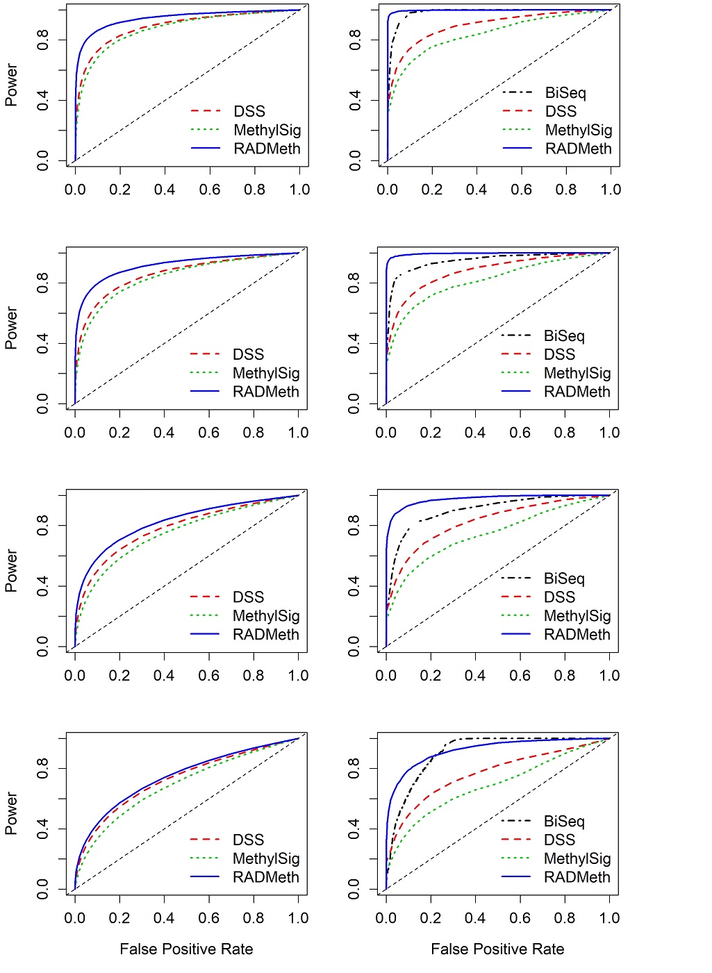
Figure 1 Comparison of mean ROC curves (averaging over 100 replicates) depicting the performance of four comparison methods for simulated WGBS data. The left column shows the results for CpG sites that were analyzed by DSS, MethylSig, and RADMeth (set R1). Note that BiSeq is not included in the comparison since it was not able to analyze these sites. The right column shows the results for CpG sites that were analyzed by all four comparison methods (set R2). The four rows show the results for the four scenarios of between-sample variability (dispersion) considered: Row 1 (Scenario 1) – (σ_G1,σ_G2) = (0, 0); Row 2 (Scenario2) – (σ_G1,σ_G2) = (0.3, 0.1); Row 3 (Scenario 3) – (σ_G1,σ_G2) = (0.7, 0.1); Row 4 (Scenario 4) – (σ_G1,σ_G2) = (1, 0.1).

Since there are almost no true DMCs among the CpG sites in the small sets of R3 (sites analyzed by all methods but RADMeth) and R4 (sites analyzed only by DSS and MethylSig; Supplementary Figure S1), no performance evaluation was carried out. These sites usually have low coverages or low methylated reads and were filtered out by RADMeth. However, since BiSeq was only able to analyze sites in R2 and R3 (covering only about 2.5% of all CpGs), we present its combined results for R2 and R3, which are similar to those for R2 only (Supplementary Figure S5).

Due to the different empirical false positive rates based on the default nominal error rates set by the different methods (Supplementary Table S2), a straightforward comparison of their power based on default settings would not be meaningful. Instead, to gain a better understanding of the relative performance of the four methods in identifying true DMCs in real data analysis, we fixed the false positive rate at 0.05 and compared the power among the methods for analyzing sites in R1 (for three methods) and R2 (all four methods). The results, shown in Table 1 (with the power being the average and the SE being the standard error of the average over 100 simulated datasets), corroborate those seen in Figure 1. That is, RADMeth had the highest power in R1 under all four scenarios, with comparable SEs among the methods. DSS slightly outperformed MethylSig, although the differences are not substantial. Note that BiSeq was not able to analyze any of the sites in R1. In R2, RADMeth remained the most powerful, although its standard errors are larger in scenarios 3 and 4 where there is a larger between-sample variability. BiSeq comes in second, but with larger variability in all four scenarios. DSS continues to outperform MethylSig in all four scenarios, with larger margins compared to those in R1. In all the methods, the SEs are larger in R2 compared to those in R1, indicating greater variability from replicate to replicate for analyzing the CpG sites in R2, as also exhibited in Supplementary Figures S2-S5. Finally, RADMeth had significantly higher power for detecting DMCs in R2 than in R1 under all four scenarios. Additionally, the powers of DSS and MethylSig in R2 are comparable to, and only slightly larger than those in R1, and in only one instance the power is smaller for MethylSig in scenario 1. The coverages for sites in R2 are similar to those in R1 but with larger variability, which possibly contributed to the different performances for different methods.

Table 1 Comparison of the average power and standard error (SE) among four methods when the false positive rate (FPR) is controlled to be 0.05 based on 100 simulated WGBS datasets.

Set R1 contains CpG sites for which BiSeq was not able to analyze, and thus no results are available.

3.3. Results From Analyzing RRBS Simulated Data

Since some of the methods (e.g, RADMeth [16]) were proposed for analyzing WGBS data while the others (e.g, BiSeq [13]) are more suitable for RRBS data, we carried out a similar study using simulated RRBS data to further evaluate the methods under a different platform. The analysis results presented below are also based on a total of 100 replicates for each of the four variability scenarios described in Section 3.1.

As with the data simulated under WGBS, the four software packages filtered out different sets of CpG sites. Since BiSeq was designed for RRBS data, it was able to retain a much larger proportion of the data for analysis. As such, for each of the four between-sample variability scenarios, about 55% of all the CpG sites were analyzed by all four methods. Nevertheless, more than 40% of the CpG sites were still filtered out by BiSeq, whereas each of the other three methods filtered out less than 5% of the sites in all four scenarios (Supplementary Figure S6).

Roughly 55% of the CpG sites were analyzed by all four methods (region R2 in Supplementary Figure S6) and the results are presented as ROC curves (Supplementary Figures S7-S10). Contrary to the results for WGBS where there was large between-replicate variability, one can see that all methods produced consistent results from replicate to replicate. For all four methods, the performance degrades somewhat and has slightly larger between-replicate variability as the between-sample variability gets larger (from scenarios 1 to 4), which is consistent with the WGBS results. For the CpG sites in R1 that were analyzed only by three methods (MethylSig, RADMeth, and DSS), the results are consistent from replicate to replicate, which is also consistent with the WGBS results (Supplementary Figures S7-S9).

Comparing among the three methods for analyzing the CpG sites in R1, one can see that based on the mean ROC curves, RADMeth has the largest AUCs in all scenarios of dispersion, whereas DSS and MethylSig are more similar to each other, with DSS slightly edging out MethylSig (Figure 2, left column). The relative performances for analyzing CpG sites in R2 among these three methods follow the same order, although DSS is appreciably better than MethylSig in the two scenarios (3 and 4) with larger variability (Figure 2, right column). These results are almost a mirror image of those from the WGBS study; therefore, regardless of the data generation platform (WGBS or RRBS), there is a consistent ordering of the performance of the methods. Not surprisingly, BiSeq rivals RADMeth as the best performer (with notably almost identical ROCs) in R2 for the first two scenarios, as it was specifically designed for analyzing RRBS data. However, as the dispersion increases, the performance of BiSeq degrades quickly (Figure 2, last two rows of right column). Once again, the BiSeq result for the combined set of R2 and R3 is similar to that for R2 only (Supplementary Figure S10).

In summary, we observe that for all methods, the power for detecting DMCs is higher for the CpG sites in R2 than in R1, indicating that those in R2 (sites not filtered out by any of the methods) have better characteristics than those in R1 (sites filtered out by BiSeq) for RRBS data (Table 2, Figures 2 and S7-9). In particular, for DSS and MethylSig, the margin of improvement from R1 to R2 is much more for RRBS than for WGBS (comparing Tables 1 and Tables 2). This is possibly due to another contributing factor, different read coverages, as those for sites in R2 are considerably larger than those in R1. Although BiSeq was designed for analyzing RRBS data and was able to retain more than 50% of the CpG sites for differential analysis, its power is only comparable to DSS with larger dispersion of underlying methylation probabilities between samples, especially given its large SEs (Tables 2). As a final comment, we note that the results from the RRBS simulated data are a bit better than those from WGBS. This is most likely due to the different profiles of the different real datasets our simulation studies are based on. Indeed, the mean or median distances between neighboring sites that are within “clusters” (neighboring sites more than 200 bp apart are treated as in different clusters) are much smaller in RRBS than in WGBS, leading to greater information sharing from RRBS data due to spatial correlation.

Table 2 Comparison of average power and standard error (SE) among four methods when the false positive rate (FPR) is controlled to be 0.05 based on 100 simulated RRBS datasets.

Set R1 contains CpG sites for which BiSeq was not able to analyze, and thus no results are available.

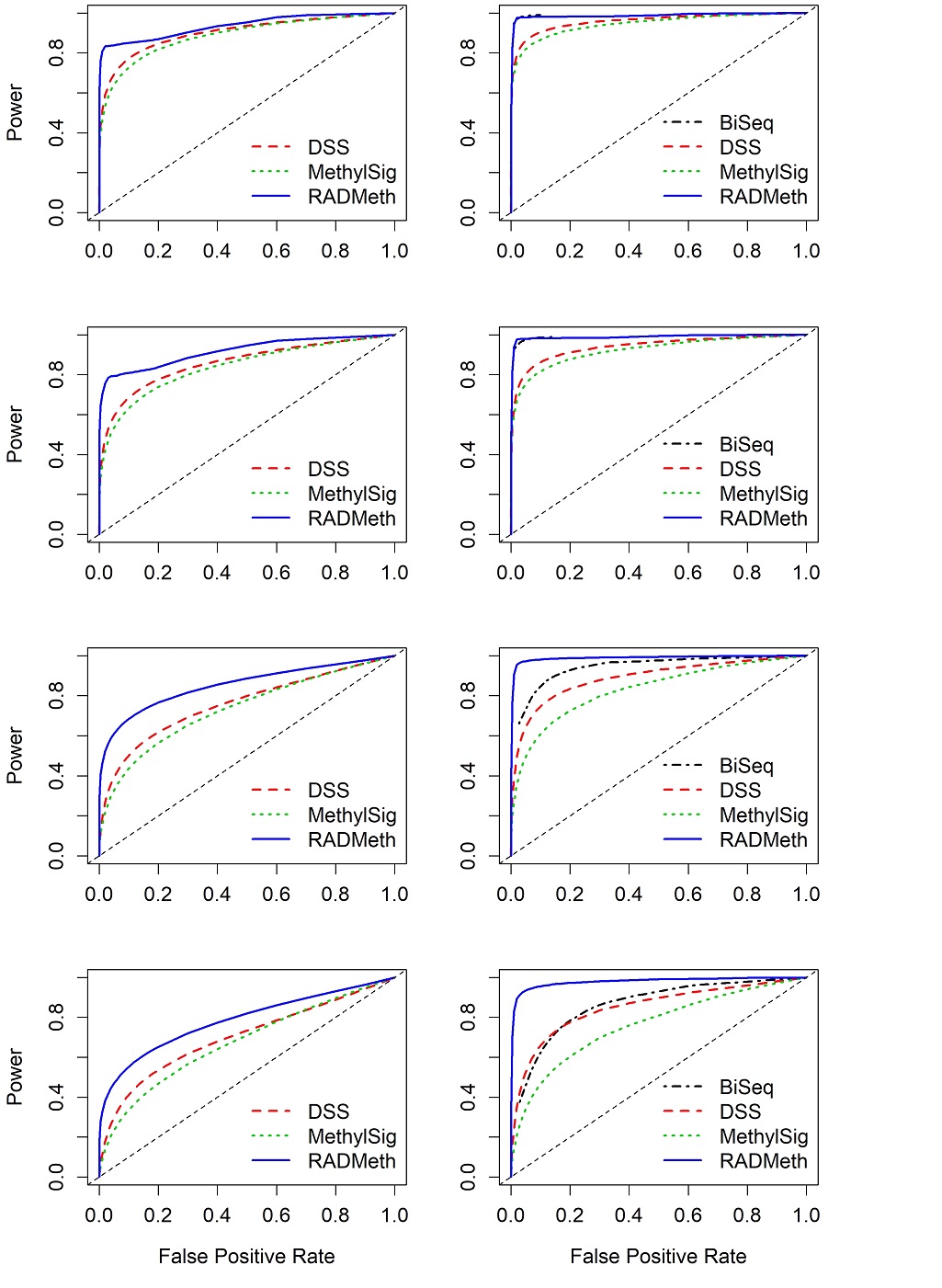
Figure 2 Comparison of mean ROC curves (averaging over 100 replicates) depicting the performance of four comparison methods for simulated RRBS data. The left column shows the results for CpG sites that were analyzed by DSS, MethylSig, and RADMeth (set R1). Note that BiSeq is not included in the comparison since it was not able to analyze these sites. The right column shows the results for CpG sites that were analyzed by all four comparison methods (set R2). The four rows show the results for the four scenarios of between-sample variability (dispersion) considered: Row 1 (Scenario 1) – (σ_G1,σ_G2) = (0, 0); Row 2 (Scenario2) – (σ_G1,σ_G2) = (0.3, 0.1); Row 3 (Scenario 3) – (σ_G1,σ_G2) = (0.7, 0.1); Row 4 (Scenario 4) – (σ_G1,σ_G2) = (1, 0.1).

4. Analyses of Two Real Data Sets

We further evaluated the four methods by applying them to two real data sets, one generated using WGBS and one based on RRBS. The understanding of pros and cons and relative performances of the methods gained through this extensive simulation study enables us to interpret the results from the real data analyses, even though there are no gold standards in these situations.

4.1. Analysis of RRBS Data From AML Patients

Data description. Our first dataset was from an acute myeloid leukemia (AML) study [29], in which four samples belonging to the AML1/ETO fusion subgroup were available. We compared the RRBS methylation profiles of these AML samples to those of four normal CD34+ bone marrow cells [15]; our goal in this data analysis was to identify differential methylation between the AML samples and the normal samples. A total of 4,642,304 CpG sites throughout the genome were considered; their distribution over the chromosomes is provided in Supplementary Table S3.

Results. The four packages with their respective default settings were used to analyze the data; using default settings is typically practiced in real data analyses and thus followed in our study to make the settings as close to real data analyses as possible. The numbers of DMCs detected were 2854, 49955, 51783, and 167545, for BiSeq, DSS, MethylSig, and RADMeth, respectively. These values vary a great deal from method to method, with BiSeq detecting the least number of DMCs; this is not surprising given what we have observed in the simulation study. The fact that DSS and MethylSig identify relatively similar numbers of DMCs (relative to the other two methods) while RADMeth detected the most is also consistent with our observation from the simulation study; therefore, the power of DSS and MethylSig are similar while RADMeth is considerably more powerful in all scenarios of sample overdispersion. The Venn diagram detailing the distributions of the detected DMCs is given in Supplementary Figure S11, including the overlapping regions among subsets of these four methods. In all, only 133 DMCs were detected by all four methods, mainly due to the small number of DMCs detected by BiSeq. In contrast, the other three methods identified more than 10,000 common DMCs. Moreover, RADMeth and DSS detected over 30,000 common DMCs, representing over 60% of the DMCs detected by DSS, which is notably a very large overlap.

Since nearby CpG sites are correlated and a DMR is the unit that is more closely tied to biological conditions [17], we also consider the number of DMRs detected by each of the methods as described in Section 2, which are 252, 2,254, 38,618, and 29,723, for BiSeq, DSS, MethylSig, and RADMeth, respectively. Note that although there are more DMCs detected by RADMeth compared to MethylSig, the converse is true for DMRs, reflected in the fact that the DMR regions in RADMeth can be much larger than those of the MethylSig, and contains many more DMCs (Supplementary Tables S4 and S5). In fact, all DMR regions detected by MethylSig are 25 bp long by design (this default value was used for this study, but it can be changed by the user) [15]. Therefore, although the size of DMRs can have biological significance, it is difficult to draw inference if the size is determined by the procedure itself. Next, we investigated the pairwise overlapping DMRs called by each pair of the four methods (Supplementary Table S6). Specifically, for the DMRs called by a package, we discerned how many of them overlap with DMRs called by another package. For example, only 7.9% of the BiSeq DMRs overlap with DMRs detected by DSS (first row of Supplementary Table S6). Here, a DMR detected by BiSeq is said to be overlapped with DMRs detected by DSS if the intersection of the particular BiSeq DMR and any of the DSS DMRs is nonempty. Hence, the concept of overlapping is not symmetrical; rather, it depends on the “base” DMRs. From Supplemental Table S5, one can see that the DMRs detected by BiSeq have smaller overlaps with those detected by the other three methods. On the other hand, 93.6% and 96.1% of the DMRs detected by DSS overlap with the DMRs detected by MethylSig and RADMeth, respectively, showing that MethylSig and RADMeth detected DMRs that are nearly supersets of DSS. Finally, although MethylSig and RADMeth also have significant overlaps, there are also large proportions of DMRs detected only by each of the two methods individually.

To further evaluate the performances of the methods and their packages and to compare and contrast them in terms of the biological relevance of the DMRs identified, we carried out a pathway analysis. First, we mapped DMRs into genes using Annovar [30], which resulted in 320, 1955, 10207, and 7047 genes for BiSeq, DSS, MethylSig, and RADMeth, respectively, although the number of genes implicated by all four methods is only 114 (Figure 3). Additionally, between DSS and RADMeth, 1927 common genes were detected, representing over 98% of the genes implicated by DSS. MethylSig and RADMeth also have a large number of common genes (6229), representing over 88% of the genes in RADMeth. Thus, at the gene level, there is a great deal of consistency among the methods, excluding BiSeq. Finally, among the 55 genes that have been implicated to be associated with AML based on the KEGG database [31], 6, 35, and 24 of them are within the set of genes inferred by DSS, MethylSig and RADMeth, respectively. Note that none of the 55 AML-associated genes were detected by BiSeq. Additionally of note, mapping using Annovar obtains genes that contain DMRs either in the gene body or within 1000 bases upstream or downstream of genes. Therefore, our analysis has included genes with DMRs in its regulatory region.

Figure 3 Venn Diagram of DMRs inferred from the four comparison methods when they were applied to analyze the AML RRBS data.

Pathway analysis was then conducted to further evaluate the relevance of the genes (using ReactomePA [32]). All genes mapped by Annovar were used in the analysis without filtering. A number of pathways were found to be significantly enriched with genes implicated by the methods (Figure 4). In particular, “developmental biology” is the common pathway among all methods, which appears to be biologically relevant for this particular study: AML is caused by cancer stem cells, where “developmental biology” plays an important role in terms of cell differentiation. Further, “axon guidance” is another common pathway detected by three of the methods (DSS, MethylSig, and RADMeth); this is also biologically relevant because this particular pathway is important for switching between cancer stem cells and non-cancer stem cells [33]. However, we note that despite the great concordance in the gene-level analysis, there are considerable discrepancies at the DMR level as we discussed above and show in Supplementary Table S6. Additional pathway analysis by considering subsets of genes inferred from at least two methods were also conducted (Supplementary Figure S12). We further conducted pathway analysis of the four sets of genes based on the KEGG database in an attempt to identify diseased pathways rather than simply considering canonical pathways. Among the 10 pathways labeled by KEGG to be important for the development of AML, MethylSig and RADMeth identified two: “Pathway in cancer” and “PI3K-Akt Signaling pathway”, while DSS only identified the latter. Note that BiSeq did not identify any since, as commented earlier, none of the 55 AML-associated genes in the KEGG database were detected by BiSeq.

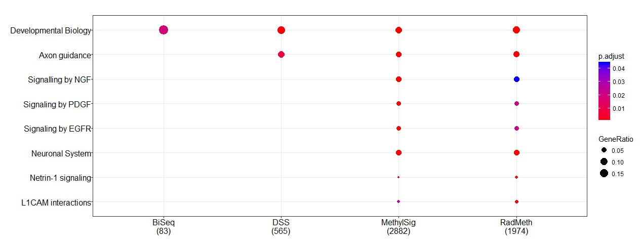
Figure 4 Pathways that are enriched with genes identified from the comparison methods when applied to the AML RRBS data.

4.2. Analysis of WGBS Mouse Brain Data

Data description. We considered the mouse brain WGBS data [34], with the goal of identifying differential methylation between neuronal and non-neuronal cells from the frontal cortex of the mouse. In the experiment, two groups (neurons versus non-neurons) of three mice each were considered. For each mouse, its age was also known, which was used as a covariate in the RADMeth analysis (3 levels). A total of 21,342,779 CpG sites were considered; their distribution over the chromosomes is provided in Supplementary Table S7. Being a WGBS dataset, the number of CpGs in this study is several times of that of the RRBS data analyzed in the previous section.

Results. We performed similar analyses as those in Section 4.1 to dissect the performance of the comparison methods. Again, the default settings of the packages were used. Like the AML data, the numbers of DMCs detected vary a great deal from method to method (Supplementary Figure S13). Although BiSeq detected the least number of DMCs, it is surprising to see that it detected more DMCs that are in common with the other methods compared to the RRBS AML data, which is contrary to what we saw in the simulation study. That being said, the overlap between BiSeq and any of the other three software packages is only a small proportion of the sites detected by the other methods (the most is at 2.44% with DSS). On the other hand, there is a large number of common DMCs among the other three methods as in the AML study. For instance, RADMeth and DSS detected over 300,000 common DMCs, representing over 94% of the DMCs detected by DSS. In terms of DMRs, BiSeq, DSS, MethylSig, and RADMeth identified 8842, 29113, 402279, and 762536 DMRs, respectively (Supplementary Table S8). As expected, these numbers are many times larger than the corresponding ones in the RRBS study; the fold change in the number of DMRs is especially large for BiSeq. With the larger number of DMRs detected by BiSeq, the overlapping percentages are 19.0%, 9.2%, and 82.9% with those detected by DSS, MethylSig, and RADMeth, respectively, compared to 7.9%, 46.0%, and 59.9% for the RRBS data (Table S5). It is interesting to see that there is a large decrease in BiSeq’s overlapping percentage with MethylSig while there is a large increase with RADMeth when comparing the results between the WGBS and RRBS data. In contrast, although there are still considerable overlaps among the other three methods, the corresponding overlapping percentages for many decrease compared to the RRBS data (see caption of Table S5). However, there are a few exceptions, especially for the DMRs detected by DSS: practically all the DMRs detected by DSS are also detected by RADMeth. For completeness, we also provide the distributions of the size (in base-pairs) of the DMRs and the number of DMCs within each DMR for each of the four methods (Supplementary Tables S9 and S10), which shows similar characteristics as in the RRBS analysis; in particular, DSS and RADMeth generally have larger regions and more DMCs within each DMR.

The DMRs identified by BiSeq, DSS, MethylSig, and RADMeth were respectively mapped to 4343, 9689, 19473, and 22374 genes using the Annovar software [30]. First, we note that BiSeq identified many more genes for this WGBS mouse brain dataset compared to the RRBS AML dataset. We can also see that a total of 3232 genes were detected by all four methods (Figure 5), a very significant number compared to only 114 in the AML study. Analysis of this common set of genes as well as genes inferred from at least two methods led to the identification of several pathways that are significantly enriched (Supplementary Figure S14).

Figure 5 Venn Diagram of DMRs inferred from the four comparison methods when they were applied to analyze the mouse brain WGBS data.

5. Discussion

In this paper, we carried out a head-to-head comparison of four methods by analyzing BS-seq data, which are typically quite limited in the sample size and show variability from sample to sample. As such, the four methods selected are beta-binomial based, as they were developed precisely to address these two specific issues. Our evaluation was objective in that the simulation study data were generated independent of any of the software packages implementing these methods. In particular, the simulation study was designed to mimic real data with limited sample sizes for both WGBS and RRBS experiments. Further, none of the real data sets used in our investigation were produced by the investigators who developed the methods being compared. We additionally note that although all four methods could be used to detect DMCs with data of context other than CpG (such as CHG and CHH, where H denotes A, T, or C), DSS and BiSeq were not designed to evaluate non-CpG data. In addition, due to low methylation levels of data in the context of CHH, BiSeq might filter out such sites before the DMC analysis, even if non-CpG data were considered.

Based on results from the extensive simulation study and analyses of both the RRBS and WGBS data, we observed that RADMeth had the most power to identify DMCs and DMRs, although its false positive rates may be a bit higher than some of the other methods. Our real data analyses also reveal that RADMeth was able to uncover biologically meaningful genes in relevant pathways. DSS also performed well for both simulated and real data; biologically meaningful pathways were identified as well. Despite its performance being slightly less stellar than that of RADMeth, its computational efficiency is an extremely attractive feature. Indeed, the analysis time for a single replicate of the WGBS simulated data shows that DSS ran more than twice as fast as RADMeth (Supplementary Table S11). MethylSig also performed well for the simulated WGBS data and had similar run time as DSS (Supplementary Table S11), although its analysis of the mouse WGBS data did not recover DMRs that were found by both RADMeth and DSS. Its performance for the RRBS data was also not as good as the other two methods, although still quite similar in some scenarios. The intersection of the gene set identified by MethylSig with that from RADMeth in the RRBS AML data did lead to enriched pathways that are related to the trait being considered.

We note that, in the absence of covariates and without invoking the respective “smoothing” or “window-based” procedures (i.e. not combining data from neighboring CpG sites in MethylSig and not combining p-values in RADMeth), MethylSig and RADMeth employ identical models, with the only difference being the respective approximation procedure for estimating the parameters of the beta-binomial distribution. As such, it is interesting to investigate under this restricted setting whether the results from these two software packages are comparable. To this end, we carried out additional analyses using the same WGBS and RRBS simulated data (where there were no covariates) but without invoking the respective “smoothing” or “window-based” procedures. The results (shown in Supplementary Figures S15 and S16) are quite close under all settings, indicating that the different approximate procedures for parameter estimation have little effects on the outcome, which is reassuring. Thus, we believe that the different procedures for borrowing information from neighboring sites are major contributors to the different performances of the two methods.

On the other hand, BiSeq was difficult to run due to its two-step FDR control procedure, especially for WGBS data, and was extremely time-consuming compared to the other methods (Supplementary Table S11). In particular, for the simulated data, if one would control the FDR in the first step in any meaningful way (e.g. setting the threshold to be less than 0.2), then no DMCs would result. The most detrimental effect though, is that almost half of the CpG sites are filtered out even for RRBS data for which BiSeq was designed, including many which are true DMCs. This is done prior to the differential analysis, leading to extremely low detection rate of true DMCs. In regard to the AML study with the RRBS data for which BiSeq was designed, it is quite surprising to see that the analysis of the data did not lead to genes that are in known biological pathways for AML. That being said, we note that a different study concluded that both BiSeq and RADMeth outperform several other methods [20]. As such, further investigation may be necessary to fully ascertain the settings in which BiSeq excels. In this study, we carried out a preliminary exploration but were unable to identify settings in which BiSeq outperformed the other methods. More specifically, we simulated data using the protocol provided in RADMeth [16], which matches up well with the BiSeq clustering criterion. The results were similar to those presented in Section 3: BiSeq was only able to analyze a small percentage of the sites, and among those that BiSeq was able to analyze, it did perform well (Supplementary Table S12).

Based on the results from our evaluation, it does not appear that a single software would uniformly dominate all the others, especially when computational efficiency is also taken into account. However, RADMeth would be recommendable since it has the best overall performance based on the simulation study. Due to the difficulty of controlling the two-step error rates and its computational intensiveness, BiSeq is not recommended until further improvements or clarifications can be made. Our experience from the real data analyses lends itself to a further recommendation that if resources permit, it might be beneficial to run all the other three software packages, as certain intersections of the genes identified appear to enrich pathways that are biologically relevant for the traits being investigated.  

This, of course, is not the first study to compare several methods, but our comparisons differ from existing ones and to the best of our knowledge, this is the first study that compares these four beta-binomial based methods head-to-head. Indeed, RADMeth was compared to DSS [16], but there does not appear to be any comparison between DSS, MethylSig, and BiSeq. As mentioned earlier, this is a completely objective study without bias toward or against any of the software, as the simulation data were not generated based on the model of any of the comparison methods. Most importantly, this study is comprehensive; it examines both simulated and real data as well as considering both the WGBS and RRBS platforms.

There are other methods and software packages for analyzing BS-seq data, including a list of 22 methods reviewed in a recent paper [23]. Methods reviewed therein not only contain those that are beta-binomial based, but also methods that are based on hidden Markov model [35,36] or Shannon entropy [37,38,39]. To be sufficiently focused in this study, we selected only four methods that are beta-binomial based as this particular type of model is a popular choice to manage both between-sample variability and small sample size with BS-seq data. As we alluded to in our analysis and the presentation of the results, borrowing information from nearby CpG sites (“smoothing”) may lead to improvement of signal strengths because closely located methylation signals are correlated [4]. As such, it would be of interest to carry out a separate study to compare methods that take such correlated signals into consideration. A related issue that warrants investigation of its own is whether direct detection of DMRs is meritorious compared to two-step approaches in which DMCs found in the first step are merged into DMRs in the second step, which is a feature in three of the four methods being compared.

Author Contributions

These authors contributed equally to this work.

Competing Interests

The authors have declared that no competing interests exist.

References

- Phillips T. The role of methylation in gene expression. Nat. Educ. 2008; 1: 116.
- Feinberg AP, Vogelstein B. Hypomethylation distinguishes genes of some human cancers from their normal counterparts. Nature. 1983; 301: 89. [CrossRef]
- Jones PA, Baylin SB. The fundamental role of epigenetic events in cancer. Nat. Rev. Genet. 2002; 3: 415. [CrossRef]
- Eckhardt F, Lewin J, Cortese R, Rakyan VK, Attwood J, Burger M, et al. DNA methylation profiling of human chromosomes 6, 20 and 22. Nat. Genet. 2006; 38: 1378. [CrossRef]
- Hoffmann MJ, Schulz WA. Causes and consequences of DNA hypomethylation in human cancer. Biochem. Cell Biol. 2005; 83: 296-321. [CrossRef]
- Madakashira BP, Sadler KC. DNA methylation, nuclear organization, and cancer. Front. Genet. 2017; 8: 76. [CrossRef]
- Tirado-Magallanes R, Rebbani K, Lim R, Pradhan S, Benoukraf T. Whole genome DNA methylation: beyond genes silencing. Oncotarget. 2017; 8: 5629. [CrossRef]
- Shukla S, Kavak E, Gregory M, Imashimizu M, Shutinoski B, Kashlev M, et al. CTCF-promoted RNA polymerase II pausing links DNA methylation to splicing. Nature. 2011; 479: 74. [CrossRef]
- Paksa A, Rajagopal J. The epigenetic basis of cellular plasticity. Curr. Opin. Cell Biol. 2017; 49: 116-122. [CrossRef]
- Robinson MD, Kahraman A, Law CW, Lindsay H, Nowicka M, Weber LM, et al. Statistical methods for detecting differentially methylated loci and regions. Front. Genet. 2014; 5: 324. [CrossRef]
- Susan JC, Harrison J, Paul CL, Frommer M. High sensitivity mapping of methylated cytosines. Nucleic Acids Res. 1994; 22: 2990-2997. [CrossRef]
- Yang Y, Sebra R, Pullman BS, Qiao W, Peter I, Desnick RJ, et al. Quantitative and multiplexed DNA methylation analysis using long-read single-molecule real-time bisulfite sequencing (SMRT-BS). BMC Genomics. 2015; 16: 350. [CrossRef]
- Hebestreit K, Dugas M, Klein H-U. Detection of significantly differentially methylated regions in targeted bisulfite sequencing data. Bioinformatics. 2013; 29: 1647-1653. [CrossRef]
- Feng H, Conneely KN, Wu H. A Bayesian hierarchical model to detect differentially methylated loci from single nucleotide resolution sequencing data. Nucleic Acids Res. 2014; 42: e69-e69. [CrossRef]
- Park Y, Figueroa ME, Rozek LS, Sartor MA. MethylSig: a whole genome DNA methylation analysis pipeline. Bioinformatics. 2014; 30: 2414-2422. [CrossRef]
- Dolzhenko E, Smith AD. Using beta-binomial regression for high-precision differential methylation analysis in multifactor whole-genome bisulfite sequencing experiments. BMC Bioinformatics. 2014; 15: 215. [CrossRef]
- Hansen KD, Langmead B, Irizarry RA. BSmooth: from whole genome bisulfite sequencing reads to differentially methylated regions. Genome Biol. 2012; 13: R83. [CrossRef]
- Park J, Lin S. Detection of Differentially Methylated Regions Using Bayesian Curve Credible Bands. Stat. Biosci. 2018; 10: 20-40. [CrossRef]
- Qin Z, Li B, Conneely KN, Wu H, Hu M, Ayyala D, et al. Statistical challenges in analyzing methylation and long-range chromosomal interaction data. Stat. Biosci. 2016; 8: 284-309. [CrossRef]
- Klein H-U, Hebestreit K. An evaluation of methods to test predefined genomic regions for differential methylation in bisulfite sequencing data. Brief. Bioinform. 2016; 17: 796-807. [CrossRef]
- Huh I, Wu X, Park T, Yi SV. Detecting differential DNA methylation from sequencing of bisulfite converted DNA of diverse species. Brief. Bioinform. 2017. [CrossRef]
- Yu X, Sun S. Comparing five statistical methods of differential methylation identification using bisulfite sequencing data. Stat Appl Genet Mol Biol. 2016; 15: 173-191. [CrossRef]
- Shafi A, Mitrea C, Nguyen T, Draghici S. A survey of the approaches for identifying differential methylation using bisulfite sequencing data. Brief. Bioinform. 2017.
- Wang H-Q, Tuominen LK, Tsai C-J. SLIM: a sliding linear model for estimating the proportion of true null hypotheses in datasets with dependence structures. Bioinformatics. 2010; 27: 225-231. [CrossRef]
- Park Y, Wu H. Differential methylation analysis for BS-seq data under general experimental design. Bioinformatics. 2016; 32: 1446-1453. [CrossRef]
- Griffiths D. Maximum likelihood estimation for the beta-binomial distribution and an application to the household distribution of the total number of cases of a disease. Biometrics. 1973: 637-648. [CrossRef]
- Hansen KD, Timp W, Bravo HC, Sabunciyan S, Langmead B, McDonald OG, et al. Increased methylation variation in epigenetic domains across cancer types. Nat. Genet. 2011; 43: 768. [CrossRef]
- Schoofs T, Rohde C, Hebestreit K, Klein H-U, Göllner S, Schulze I, et al. DNA methylation changes are a late event in acute promyelocytic leukemia and coincide with loss of transcription factor binding. Blood. 2013; 121: 178-187. [CrossRef]
- Rampal R, Alkalin A, Madzo J, Vasanthakumar A, Pronier E, Patel J, et al. DNA hydroxymethylation profiling reveals that WT1 mutations result in loss of TET2 function in acute myeloid leukemia. Cell Rep. 2014; 9: 1841-1855. [CrossRef]
- Wang K, Li M, Hakonarson H. ANNOVAR: functional annotation of genetic variants from high-throughput sequencing data. Nucleic Acids Res. 2010; 38: e164-e164. [CrossRef]
- Kanehisa M, Araki M, Goto S, Hattori M, Hirakawa M, Itoh M, et al. KEGG for linking genomes to life and the environment. Nucleic Acids Res. 2007; 36: D480-D484. [CrossRef]
- Yu G, He Q-Y. ReactomePA: an R/Bioconductor package for reactome pathway analysis and visualization. Mol. Biosyst. 2016; 12: 477-479. [CrossRef]
- Yamazaki J, Estecio MR, Lu Y, Long H, Malouf GG, Graber D, et al. The epigenome of AML stem and progenitor cells. Epigenetics. 2013; 8: 92-104. [CrossRef]
- Lister R, Mukamel EA, Nery JR, Urich M, Puddifoot CA, Johnson ND, et al. Global epigenomic reconfiguration during mammalian brain development. Science. 2013; 341: 1237905. [CrossRef]
- Sun S, Yu X. HMM-Fisher: identifying differential methylation using a hidden Markov model and Fisher’s exact test. Stat Appl Genet Mol Biol. 2016; 15: 55-67. [CrossRef]
- Yu X, Sun S. HMM-DM: identifying differentially methylated regions using a hidden Markov model. Stat Appl Genet Mol Biol. 2016; 15: 69-81. [CrossRef]
- Zhang Y, Liu H, Lv J, Xiao X, Zhu J, Liu X, et al. QDMR: a quantitative method for identification of differentially methylated regions by entropy. Nucleic Acids Res. 2011; 39: e58-e58. [CrossRef]
- Liu H, Liu X, Zhang S, Lv J, Li S, Shang S, et al. Systematic identification and annotation of human methylation marks based on bisulfite sequencing methylomes reveals distinct roles of cell type-specific hypomethylation in the regulation of cell identity genes. Nucleic Acids Res. 2015; 44: 75-94. [CrossRef]
- Su J, Yan H, Wei Y, Liu H, Liu H, Wang F, et al. CpG_MPs: identification of CpG methylation patterns of genomic regions from high-throughput bisulfite sequencing data. Nucleic Acids Res. 2012; 41: e4-e4. [CrossRef]